Performance Test

The package was tested against injected random Influence coefficient matrices hsbalance.IC_matrix.Alpha with N x N size. The output can be summarized in the following plot.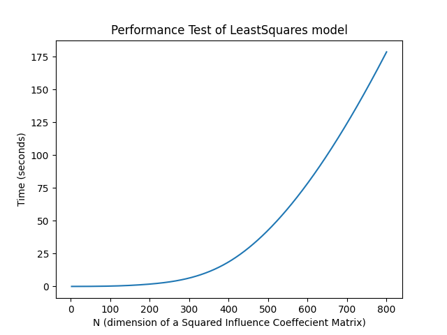

The graph was a test for the Least Squares model. It shows a good time performance of 800 x 800 matrix under 3 minutes.

The hardware and software for the machine running the test can be found data/test_conditions.txt

The code below is to generate the previous plot.

import time
from scipy.interpolate import make_interp_spline
import numpy as np
import matplotlib.pyplot as plt
from hsbalance import Alpha, model, tools



def test_performance(n):
    '''
    Test the performance of model time_wise.
    Args:
      n : dimension of influence coefficient matrix nxn.
    Output:
      t : time elapsed in the test rounded to 2 decimal.
    '''
    # Generate alpha matrix nxn dimension
    alpha = Alpha()
    real = np.random.uniform(0, 10, [n, n])
    imag = np.random.uniform(0, 10, [n, n])
    alpha.add(real + imag * 1j)
    # Generate initial condition A matrix nx1
    real = np.random.uniform(0, 10, [n, 1])
    imag = np.random.uniform(0, 10, [n, 1])
    A= real + imag * 1j
    # start timing
    start = time.time()
    # building model LeastSquare.
    w =  model.LeastSquares(A, alpha).solve()
    # implement the model to get run time.
    error = tools.residual_vibration(alpha.value, w, A)
    t = time.time() - start
    return round(t, 2)
performance_time = []
N = [2, 10, 50, 100, 200, 400, 600, 800]
for n in N:
    performance_time.append(test_performance(n))
print(N, performance_time)
spline = make_interp_spline(N, performance_time)
x = np.linspace(min(N), max(N), 500)
y  = spline(x)
plt.plot(x, y, label="Performace Test")
plt.xlabel('N (dimension of a Squared Influence Coeffecient Matrix)')
plt.ylabel('Time (seconds)')
plt.title('Performance Test of LeastSquares model')
plt.show()